First steps in Lucent 

Table of Contents

First steps in Lucent

Note

This page assumes you already have installed Lucent

Note

This page is still WIP. While it is under construction please check out the existing colab notebooks on the original project’s github main page.

Graphical interface vs. script 

Lucent can be interacted with either indirectly via the graphical interface or directly via a python script by calling the appropriate lucent.optvis methods.

When you are just starting out with interpretability we recommend having a look at the graphical interface first and then transitioning to optvis later if you want to change some of the default settings, add your own custom objective function or what have you.

Graphical Interface 

The graphical interface is still WIP, but you can check it out by running

cd $LUCENT_PATH/lucent/interface
streamlit run investigate_layer.py

This should then open a tab in your browser looking like this

You can now select a model of your choice, either from torchvision.models or upload your own model. If you wish to load from an old session, you can specify the data directory and tick the Load images from data dir checkbox.

Click Save config. Lucent should automatically detect all relevant layers for you and list them in the layer drop menu. Now you can generate the features for each layer by selecting the layer and clicking Generate Layer Features.

If you select Display Database, all of the loaded and generated images for the selected model will be displayed.

Lucent comes with a couple of predefined interfaces geared towards investigating different phenomena. You can check them out in the folder interface. ..

TODO: add link to interface folder

Lucent via Script 

We recommend using an interactive environment for this, such as your own jupyter notebook or a Google Colab.

For an interactive version, see the official, updated Colab notebook

If you are running the code in a colab, we first need to install lucent:

!pip install --quiet git+https://github.com/TomFrederik/lucent.git

Let’s import torch and lucent, and set the device variable.

import torch
from lucent.optvis import render, param, transform, objectives

device = torch.device('cuda') if torch.cuda.is_available() else 'cpu'

We will now load the InceptionV1 model (also known as GoogLeNet), but you could also use any other image-based network here. We will send it to the device and set it to eval mode to avoid gradient tracking and unnecessary computations and disable any potential dropouts.

from torchvision.models import googlenet # import InceptionV1 aka GoogLeNet

model = googlenet(pretrained=True)
_ = model.to(device).eval() # the underscore prevents printing the model if it's the last line in a ipynb cell

Feature visualization 

Now that we have our model we will start of with the bread and butter of mechanistic interpretability: feature visualization.

The core idea is to optimize the input image to the network such that a certain neuron or channel gets maximally excited.

Question

How would that help with understanding what network is doing? How could that give us misleading results?

Answer

Optimizing the input to maximally excite a neuron produces a sort of super-stimulus. It establishes one direction of causality, i.e. … #TODO

However, this method usually produces images that are very different from the data distribution. We might be worried that it picks up on spurious correlations instead of reflecting what the neuron does when it encounters real images.

In order to perform feature visualization we have to specify an objective function with respect to which we will optimize the input image.

The default of render.render_vis is to assume you gave it a description of the form ‘layer:channel’ and want it to optimize the whole feature map of the channel.

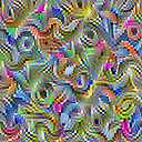
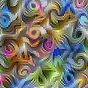
For example, if we want to optimize the input for the 476th channel in layer inception4a:

# list of images has one element in this case
list_of_images = render.render_vis(model, "inception4a:476")

Now, what if you don’t know the names of all the layers in your network? Lucent has you covered, with its get_model_layers method:

from lucent.model_utils import get_model_layers, filter_layer_names

layer_names, dependency_graph = get_model_layers(model)

print(filter_layer_names(layer_names, depth=1))

['conv1', 'conv1->conv', 'conv2', 'conv2->conv', 'conv3', 'conv3->conv', 'inception3a', 'inception3a->branch1', 'inception3a->branch1->conv', ...]

layer_names is a list of all layer names, including nested ones. Nesting is denoted via layer->sublayer. dependency_graph makes this parent-child relation more explicit by storing all layers in a nested OrderedDict.

At the present moment we haven’t implemented a method to detect how many channels each layer has, but that’s upcoming.

Objectives 

What loss function do we want to minimize?

Or from another point of view, what part of the model do we want to understand?

In essence, we are trying to generate an image that causes a particular neuron or filter to activate strongly. The objective allows us to select a specific neuron, channel or a mix! The default is the channel objective.

You can also explicitly state the objective instead of providing an identifying string:

# This code snippet is equivalent to what we did above
obj = objectives.channel('inception4a', 476)
list_of_images = render.render_vis(model, obj)

There are a few predefined objective functions, such as channel, neuron and direction. Learn more about them in Native Objectives. You can also define your own objective, which we will explain in Custom Objectives.

In principle, the objective can be any differentiable function that takes as input the feature map of the entire model and returns some loss value. For example, by using the channel objective, we specify that we want to minimize the negative, mean activation of a particular layer’s activation at a particular channel.

Objectives can be combined via all the standard arithmetic operators (+, -, *, /).

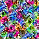
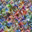
For example, we could jointly optimize two channels to see the interaction of two neurons:

obj = objectives.channel(476) + objectives.channel(465)
list_of_images = render.render_vis(model, obj)

Summation

If you want to use the sum operator, the built-in python method results in an unfortunate nested description. To circumvent this, you can use the staticmethod Objective.sum(iterable_of_objectives) instead.

Parameterizations 

We said above that feature visualization is all about optimizing the input image for a given objective function. But in order to that via the typical autodiff machinery, we need to parameterize the image somehow. This way we can then optimize the parameters of that image.

Question

Can you come up with at least two ways of parameterizing an image?

Answer

The first approach is to simply use an RGB parameterization. That is, for every pixel in the image, we store three float values between 0 and 1 representing the R-, G-, and B-value respectively.

The second approach is to switch to a fourier representation of the image. The parameters are then the coefficients of the different fourier basis functions. This approach does actually produce nicer representations than the RGB parameterization which tends to have certain grainy, high-frequency patterns.

There are more possible approaches. You can find out about them on the Parameterizations page.

In order to tell render_vis our parameterization we can use the param_f keyword. param_f should be a function without arguments that returns the image tensor.

The canonical way to do this in Lucent is to call lucent.param.image:

# the width parameter determines the image width -> influences runtime significantly
# this is vanilla RGB-parameterization
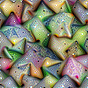
param_f = lambda: param.image(w=128, fft=False, decorrelate=False)

# using Fourier basis instead of pixel values
fft_param_f = lambda: param.image(w=128, fft=True, decorrelate=False)

# this is the default setting
fft_decor_param_f = lambda: param.image(w=128, fft=True, decorrelate=True)

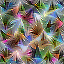
# Let's see what the difference in output is:
images = []
for f in [param_f, fft_param_f, fft_decor_param_f]:
    images.append(render.render_vis(model, 'inception4a:476', param_f=f))

Batching 

Let’s say you want to generate many visualizations at once, either for different settings and the same objective or different objectives.

The way Lucent handles this is a bit unintuitive in the beginning.

In essence, you can specify for each objective function which batch dimension it should pay attention to. By default, an objective is applied to the full batch of images, but you can also pass a batch parameter to specify which element of the batch it should be applied to. (Anything in between one element and all elements is not support at the moment.)

So.. what does this mean for our parameterization function? We have to make sure that the returned images also have a batch dimension. If you are using the built-in parameterizations, you can simply pass this as an additional parameter:

batch_size = 3
param_f = lambda: param.image(w=128, batch=batch_size)

Now, let’s say we want to optimize three different channels, 476, 477, and 478 of the layer inception4a. We do this by creating the sum of the individual objectives and setting the batch keyword argument to a different value in [0,1,2] for each of them. This way, each objective will only be applied to the i-th image, and we can optimize them in parallel.

objective = objectives.Objective.sum(objectives.channel('inception4a', ch, batch=i) for i, ch in enumerate([476, 477, 478]))
list_of_images = render.render_vis(model, objective, param_f=param_f) # list_of_images has length 3

Transformations 

Next to parameterizing the image via the frequency domain, another trick to reduce high-frequency patterns in the visualization is to impose robustness of the result under certain transformations that are applied to the input.

Those transformations could be paddings, small translations (jitter), rescaling and rotating, just to name a few.

The default setting for render_vis is given by

standard_transforms = [
    pad(12, mode="constant", constant_value=0.5),
    jitter(8),
    random_scale([1 + (i - 5) / 50.0 for i in range(11)]),
    random_rotate(list(range(-10, 11)) + 5 * [0]),
    jitter(4),
]

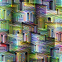
So, actually we already used transformations in all of our examples above. Let’s see what our go-to example looks like without it by passing an empty iterable:

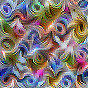
list_of_images = render.render_vis(model, 'inception4a:476', transforms=[])

Whoops, that didn’t work. Let’s see if it is better if we increase the variation in our random initialization (default is sd=0.01).

There we go! Sometimes you will get a grey image. We think this is not a bug of the library but rather that the optimizer can’t find a locally better image, especially if it does not have the transformation constraint. If this happens to you and you already tried multiple different settings create an issue on GitHub please.

In addition to the transformations above, each image is by default normalized. If you want to override this normalization you can provide a custom preprocess_f to render_vis or completely disable it with preprocess=False.

For a full ist of available transformations see Transformations.